|
Methods to Design Points on the Surface |
Scroll |
You can select a method to build a group of points using the Method group of buttons: The following options are available:
•By number of points in UV directions,
•By grid around selected point.
In the process of plotting, you can switch between methods. The values of parameters entered for each method are stored until the command is completed.
 By number of points in UV directions
The number of points in UV directions is set in the fields Number of Points, U and Number of Points, V.
The points are built in such a way so that there are N points in direction U, and M points in direction V.

The value of the maximum linear deviation is set in the Linear deviation. The field appears on the Parameter Panel if the selected face is not plane.
The points are built in such a way so that deviations of edges of the approximating polyhedron that connect the adjacent points in directions U and V from the selected surface should not exceed the specified value. The density of points located on the surface depends on its curvature: the points are denser on the segments of greater curvature, and more sparse – on the segments of less curvature.

The value of the maximum angular deviation is set in the field Angular Deviation. The field appears on the Parameter Panel if the selected face is not plane.
The points are built in such a way so that the angles between tangents to the surface at the point and edges of the approximating polyhedron that connect the point with the adjacent points in directions U and V should not exceed the specified value. The density of points located on the surface depends on its curvature: the points are denser on the segments of greater curvature, and more sparse – on the segments of less curvature.

The points are located on the theoretical surface of the selected face to create a grid around the specified point lying on the same theoretical surface. The specified point is the center of the grid.
You can use one of the following methods to set the position of the center of the grid.
•Use the mouse to drag the "Center" characteristic point to the required position on the face.
•Input the values of the U and V parameters of the grid center on the theoretical surface of the face in the UV parameters, % field.
•Specify a point object lying on the selected face within its limits. The name of the selected object is displayed in the Snap Point field.
Associativity is formed between the grid center and the point object. Due to this associativity, the grid center will follow the object when its position changes.

The grid center may be located both within the contour of the selected face and go beyond it. You can extend the theoretical surface of the face (depending on the type of the face), if required. The Figure shows examples of location of the grid center outside the contour of the selected face when different states of the Allow for Borders option. Note that if the grid center goes beyond the theoretical surface of the face, it will limit the grid in the direction of its displacement (Fig. b).
|
|
a) |
|
|
|
b) |
|
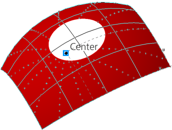
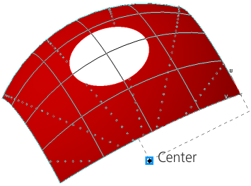
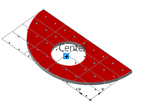
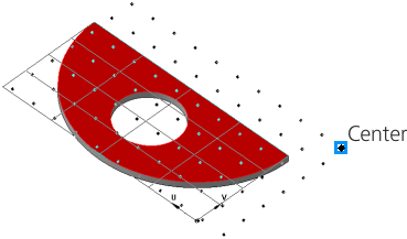
Examples of the center of the grid location outside the contour of the selected face
when plotting a point group by surface:
a) option Consider boundaries is enabled; b) option Consider boundaries is disabled
The grid may be rectangular, concentric or hexagonal. You can select the required type using the Mesh type group of buttons. Setting parameters for each type is shown in the Table.
Grid parameters controls
Grid type |
Rules for plotting |
Example |
|
|
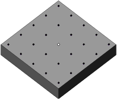
Rectangular |
This variant is available for all types of faces. The set of grid parameters depends on the type of the selected face. •If the face is plane, spherical, or cylindrical, then the step values along the first and second grid axes are specified in the Step by axis 1 and Step by axis 2 fields. •If the surface is conical, toroidal, or arbitrary, then in the fields Step by U, % and Step by V, %, the step values for the U and V parameters are specified. |
|
|
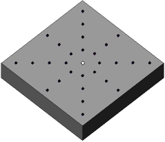
Concentric |
This variant is available, if a plane or spherical face is used for plotting. In the fields Number of Rays and Radial pitch, the number of radial rays and the radial grid step are specified. |
|
|
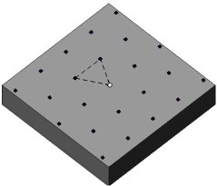
Hexagonal |
This variant is available, if a plane or cylindrical face is used for plotting. A hexagonal grid has equal pitch between adjacent grid nodes. The pitch value is set in the Step field. |
|


In the process of plotting, you can switch between types of the grid. Data entered for each type are stored until the command is completed.
If a surface of constant curvature (for example, a plane face or a sphere) is used to plot a point group, you can rotate the grid at an arbitrary angle around the face normal in the center of the grid. The angle of the grid rotation is calculated from the direction U counterclockwise.
Use the Rotation field to input the value of the rotation angle. The value can be positive – counterclockwise rotation, and negative – clockwise rotation.